Explorative Data Analysis

Tidyverse - Part 5

Otho Mantegazza

Putting it All Together

The steps of EDA

We have covered almost all steps of what is called Explorative Data Analysis (EDA).

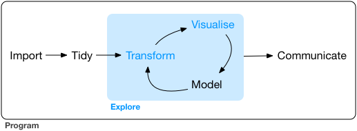
Image Source: R4DS

The Steps of EDA

The explore part is iterative.

• Transform
• Visualize
• Model

A imperative for EDA

To get insights from data that you haven’t faced before,

1. Look what’s inside.
2. Learn their structure
3. Formulate questions
4. Try to anwser them with statistical methods.

Briefly, explore them.

Practice Dataset

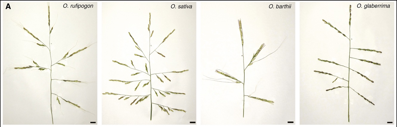
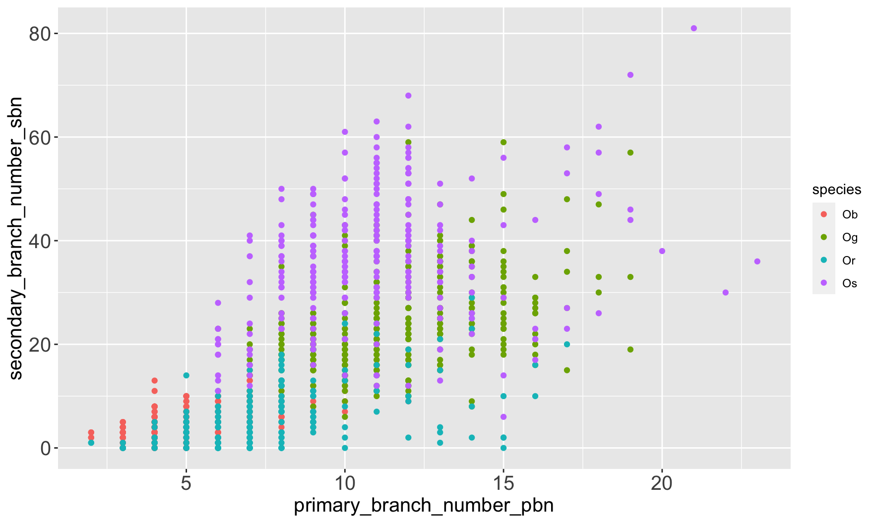
Transcriptome and Phenotype of multiple Rice species

A set of AP2-like genes is associated with inflorescence branching and architecture in domesticated rice.

• Paper
• DOWNLOAD SUPPLEMENTARY TABLE S3 - 96Kb !It’s a CSV file!

4 rice accessions

species_id	species	continent	status
Ob	Oryza barthii	African	Wild
Og	Oryza glaberrima	African	Cultivated
Or	Oryza rufipogon	Asian	Wild
Os	Oryza sativa	Asian	Cultivated

Let’s read the Data

rice <-  
   paste0('https://raw.githubusercontent.com/othomantegazza',
           '/mawazo-summer-school/main/data-int/rice.csv') %>% 
  read_delim(delim = ';') %>% 
  janitor::clean_names()

rice %>% 
  glimpse()

Rows: 1,140
Columns: 18
$ id                                                     <chr> "Ob01", "Ob01",…
$ species                                                <chr> "Ob", "Ob", "Ob…
$ accession_name                                         <chr> "B197", "B197",…
$ origine_continent                                      <chr> "Africa", "Afri…
$ type_wild_cultivated                                   <chr> "Wild", "Wild",…
$ sowing_localisation                                    <chr> "Cali-Colombia"…
$ replicate_nb_1_2                                       <dbl> 1, 1, 1, 1, 1, …
$ plant_nb_1_to_3                                        <dbl> 1, 1, 1, 2, 2, …
$ panicle_nb_1_to_3                                      <dbl> 1, 2, 3, 1, 2, …
$ rachis_length_rl_in_cm                                 <dbl> 8.10, 6.51, 4.6…
$ primary_branch_number_pbn                              <dbl> 5, 5, 4, 4, 4, …
$ average_of_primary_branch_length_in_cm_pbl             <dbl> 6.73, 6.26, 6.9…
$ average_of_internode_along_primary_branch_in_cm_pbil   <dbl> 2.03, 1.63, 1.5…
$ secondary_branch_number_sbn                            <dbl> 5, 3, 2, 5, 1, …
$ average_of_secondary_branch_length_in_cm_sbl           <dbl> 1.74, 1.51, 1.9…
$ average_of_internode_along_secondary_branch_in_cm_sbil <dbl> 0.99, 0.72, 1.6…
$ tertiary_branch_number_tbn                             <dbl> 0, 0, 0, 0, 0, …
$ spikelet_number_sp_n                                   <dbl> 38, 38, 30, 35,…

rice %>% 
  count(species, origine_continent, type_wild_cultivated)

# A tibble: 4 × 4
  species origine_continent type_wild_cultivated     n
  <chr>   <chr>             <chr>                <int>
1 Ob      Africa            Wild                   264
2 Og      Africa            Cultivated             370
3 Or      Asia              Wild                   215
4 Os      Asia              Cultivated             291

Goal of the paper

Explore the phenotypic and transcripts of panicle development.

Traits of agronomic interest in the panicle:

• Number of Spikelet,
• Number of Primary branches
• Number of Seconday branches

Let’s explore the data

rice %>% 
  ggplot(aes(x = primary_branch_number_pbn,
             y = secondary_branch_number_sbn)) +
  geom_point()

rice %>% 
  ggplot(aes(x = primary_branch_number_pbn,
             y = secondary_branch_number_sbn,
             colour = species)) +
  geom_point()

rice %>% 
  ggplot(aes(x = primary_branch_number_pbn,
             y = secondary_branch_number_sbn,
             colour = species)) +
  geom_point(alpha = .4)

rice %>% 
  ggplot(aes(x = primary_branch_number_pbn,
             y = secondary_branch_number_sbn,
             colour = species)) +
  geom_point(alpha = .4) +
  facet_wrap(facets = 'species')

rice %>% 
  ggplot(aes(x = primary_branch_number_pbn,
             y = secondary_branch_number_sbn)) +
  geom_hex(bins = c(12, 3)) +
  scale_fill_gradient(low = 'grey70', high = 'blue') +
  facet_wrap(facets = 'species')

rice %>% 
  select(species,
         primary_branch_number_pbn,
         secondary_branch_number_sbn) %>% 
  pivot_longer(-species,
               names_to = 'branch_type',
               values_to = 'branch_count') %>% 
  ggplot(aes(x = branch_type,
             y = branch_count,
             fill = species)) +
  geom_boxplot()

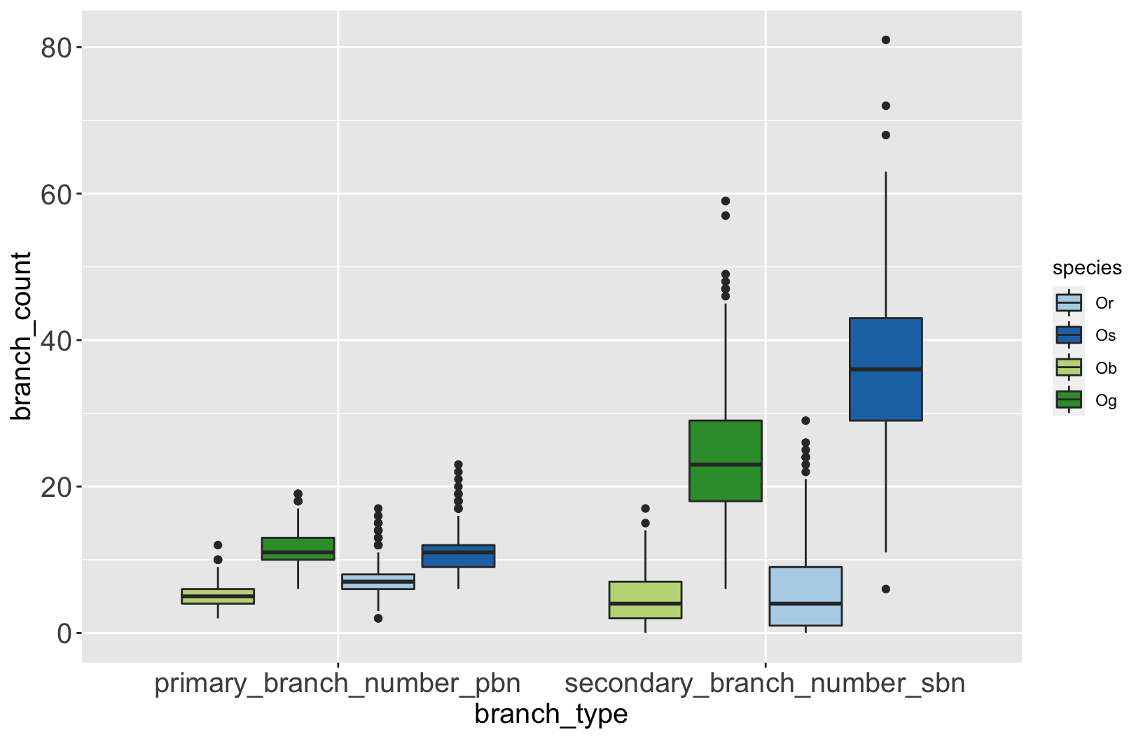
# define colors
rice_colors <- 
  c(Or = '#b5d4e9',
    Os = '#1f74b4',
    Ob = '#c0d787',
    Og = '#349a37')

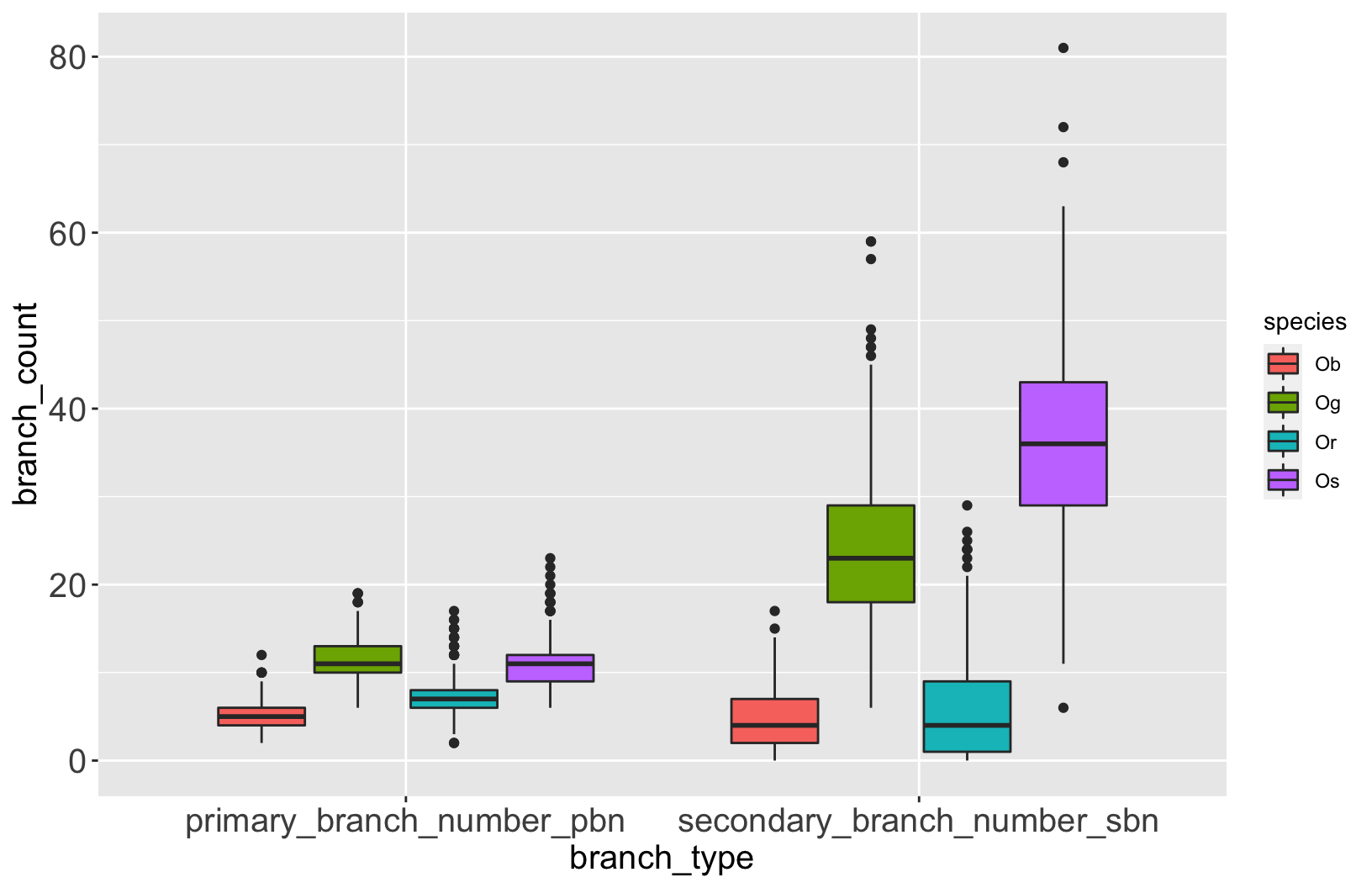
# plot
rice %>% 
  select(species,
         primary_branch_number_pbn,
         secondary_branch_number_sbn) %>% 
  pivot_longer(-species,
               names_to = 'branch_type',
               values_to = 'branch_count') %>% 
  ggplot(aes(x = branch_type,
             y = branch_count,
             fill = species)) +
  geom_boxplot() +
  scale_fill_manual(values = rice_colors)

Exercise

Explore the rice panicle dataset.

How are the measured variable distributed? Do they correlate with each other?

Can you find some of the traits that mark the differences between wild and domesticated varieties? And what about the differences between the Asian and African varieties.

Did you manage to anwser all your questions with summary statistics and graphics? Note down questions that are still open and that you think should be tackled with more advanced statistics.