Clean and Tidy Data

Tidyverse - Part 4

Otho Mantegazza

Tidy Data

Which Dataset is Tidy?

A common practical way to structure (empirical) data.

Every column is a variable.
Every row is an observation.
Every cell is a single value.
(Every observational unit is in its own table).

Plus: fixed variables should come first, followed by measured variables.

Reference: An Introduction to Tidy Data

Which Dataset is Tidy?

Source: R4DS - Tidy Data

Joey

Monica

Rachel

Phoebe

Ross

Chandler

Tribbiani

Geller

Green

Buffay

Geller

Bing

Semantics of (tidy) Data

Always quoting the Tidy Data article:

A dataset is a collection of values.
Every value belongs to a variable and an observation.
A variable contains all values that measure the same underlying attribute (like height, temperature, duration) across units.
An observation contains all values measured on the same unit (like a person, or a day, or a race) across attributes

Tools: Tidy data with Tidyr

Tidyr provides functions for:

Pivoting data.
Rectangling data.
Nesting data.
Combining and splitting columns.
Make missing values explicit.

Let’s tidy the data from Pangaea

Pangea Data

Remember the dataset from Pangaea?

pangaea_filename <- 'Dataset_S2_HCl-leaching.tab'

pangaea_path <- here('data-int/Wu-etal_2022/datasets', pangaea_filename)

pangaea_data <- 
  pangaea_path %>% 
  read_delim(delim = '\t',
             skip = 49)

pangaea_data %>% 
  glimpse()

Rows: 128
Columns: 19
$ Event                      <chr> "SL73BC", "SL73BC", "SL73BC", "SL73BC", "SL…
$ Latitude                   <dbl> 39.6617, 39.6617, 39.6617, 39.6617, 39.6617…
$ Longitude                  <dbl> 24.5117, 24.5117, 24.5117, 24.5117, 24.5117…
$ `Elevation [m]`            <dbl> -339, -339, -339, -339, -339, -339, -339, -…
$ `Sample label (barite-Sr)` <chr> "SL73-1", "SL73-2", "SL73-3", "SL73-4", "SL…
$ `Samp type`                <chr> "non-S1", "non-S1", "non-S1", "S1b", "S1b",…
$ `Depth [m]`                <dbl> 0.0045, 0.0465, 0.0665, 0.1215, 0.1765, 0.1…
$ `Age [ka BP]`              <dbl> 1.66, 3.13, 4.13, 5.75, 7.30, 7.78, 8.65, 9…
$ `CaCO3 [%]`                <dbl> 61.5, 55.1, 53.0, 43.4, 41.8, 42.3, 42.6, 3…
$ `Ba [µg/g] (Leachate)`     <dbl> 72.6, 64.3, 37.4, 63.5, 101.0, 141.0, 75.2,…
$ `Sr [µg/g] (Leachate)`     <dbl> 767, 681, 690, 552, 527, 528, 551, 482, 391…
$ `Ca [µg/g] (Leachate)`     <dbl> 188951.9, 163260.4, 162188.7, 125937.6, 124…
$ `Al [µg/g] (Leachate)`     <dbl> 10612.7, 11428.4, 5463.0, 3261.5, 2121.7, 1…
$ `Fe [µg/g] (Leachate)`     <dbl> 5935.0, 6814.3, 2465.7, 3936.8, 189.6, 7711…
$ `Ba [µg/g] (Residue)`      <dbl> 171.0, 198.0, 251.0, 290.0, 315.0, 259.0, 3…
$ `Sr [µg/g] (Residue)`      <dbl> 66.6, 71.3, 90.3, 99.8, 106.0, 90.7, 108.0,…
$ `Ca [µg/g] (Residue)`      <dbl> 2315.5, 2369.6, 3007.7, 3447.9, 3713.2, 331…
$ `Al [µg/g] (Residue)`      <dbl> 29262.5, 35561.4, 45862.4, 52485.6, 55083.0…
$ `Fe [µg/g] (Residue)`      <dbl> 14834.8, 18301.4, 24534.5, 30745.3, 28532.2…

Clean the column names with `Janitor`

we can remove capitalization, spaces, and strange characters from the column names with the function clean_names() from the Janitor Package.

pangaea_data <- 
  pangaea_data %>% 
  janitor::clean_names()

pangaea_data %>%
  glimpse()

Rows: 128
Columns: 19
$ event                  <chr> "SL73BC", "SL73BC", "SL73BC", "SL73BC", "SL73BC…
$ latitude               <dbl> 39.6617, 39.6617, 39.6617, 39.6617, 39.6617, 39…
$ longitude              <dbl> 24.5117, 24.5117, 24.5117, 24.5117, 24.5117, 24…
$ elevation_m            <dbl> -339, -339, -339, -339, -339, -339, -339, -339,…
$ sample_label_barite_sr <chr> "SL73-1", "SL73-2", "SL73-3", "SL73-4", "SL73-5…
$ samp_type              <chr> "non-S1", "non-S1", "non-S1", "S1b", "S1b", "S1…
$ depth_m                <dbl> 0.0045, 0.0465, 0.0665, 0.1215, 0.1765, 0.1915,…
$ age_ka_bp              <dbl> 1.66, 3.13, 4.13, 5.75, 7.30, 7.78, 8.65, 9.94,…
$ ca_co3_percent         <dbl> 61.5, 55.1, 53.0, 43.4, 41.8, 42.3, 42.6, 39.1,…
$ ba_mg_g_leachate       <dbl> 72.6, 64.3, 37.4, 63.5, 101.0, 141.0, 75.2, 99.…
$ sr_mg_g_leachate       <dbl> 767, 681, 690, 552, 527, 528, 551, 482, 391, 70…
$ ca_mg_g_leachate       <dbl> 188951.9, 163260.4, 162188.7, 125937.6, 124733.…
$ al_mg_g_leachate       <dbl> 10612.7, 11428.4, 5463.0, 3261.5, 2121.7, 12740…
$ fe_mg_g_leachate       <dbl> 5935.0, 6814.3, 2465.7, 3936.8, 189.6, 7711.3, …
$ ba_mg_g_residue        <dbl> 171.0, 198.0, 251.0, 290.0, 315.0, 259.0, 310.0…
$ sr_mg_g_residue        <dbl> 66.6, 71.3, 90.3, 99.8, 106.0, 90.7, 108.0, 96.…
$ ca_mg_g_residue        <dbl> 2315.5, 2369.6, 3007.7, 3447.9, 3713.2, 3316.7,…
$ al_mg_g_residue        <dbl> 29262.5, 35561.4, 45862.4, 52485.6, 55083.0, 44…
$ fe_mg_g_residue        <dbl> 14834.8, 18301.4, 24534.5, 30745.3, 28532.2, 22…

Watch out: Janitor transforms µ into m (so micrograms become milligrams).

Place fixed variables in the first columns

Which column is a fixed variable?

I’m not sure if ca_co3_percent is a measured variable, and if it belongs to another informational unit.

Besides that, the fixed variables are already in front.

There are values stored in the column names

Let’s pivot the measured variables.

pangaea_long <- 
  pangaea_data %>% 
  pivot_longer(
    cols = contains(match = c('leachate', 'residue')),
    values_to = 'concentration',
    names_to = 'element'
  )

pangaea_long

# A tibble: 1,280 × 11
   event latit…¹ longi…² eleva…³ sampl…⁴ samp_…⁵ depth_m age_k…⁶ ca_co…⁷ element
   <chr>   <dbl>   <dbl>   <dbl> <chr>   <chr>     <dbl>   <dbl>   <dbl> <chr>  
 1 SL73…    39.7    24.5    -339 SL73-1  non-S1   0.0045    1.66    61.5 ba_mg_…
 2 SL73…    39.7    24.5    -339 SL73-1  non-S1   0.0045    1.66    61.5 sr_mg_…
 3 SL73…    39.7    24.5    -339 SL73-1  non-S1   0.0045    1.66    61.5 ca_mg_…
 4 SL73…    39.7    24.5    -339 SL73-1  non-S1   0.0045    1.66    61.5 al_mg_…
 5 SL73…    39.7    24.5    -339 SL73-1  non-S1   0.0045    1.66    61.5 fe_mg_…
 6 SL73…    39.7    24.5    -339 SL73-1  non-S1   0.0045    1.66    61.5 ba_mg_…
 7 SL73…    39.7    24.5    -339 SL73-1  non-S1   0.0045    1.66    61.5 sr_mg_…
 8 SL73…    39.7    24.5    -339 SL73-1  non-S1   0.0045    1.66    61.5 ca_mg_…
 9 SL73…    39.7    24.5    -339 SL73-1  non-S1   0.0045    1.66    61.5 al_mg_…
10 SL73…    39.7    24.5    -339 SL73-1  non-S1   0.0045    1.66    61.5 fe_mg_…
# … with 1,270 more rows, 1 more variable: concentration <dbl>, and abbreviated
#   variable names ¹latitude, ²longitude, ³elevation_m,
#   ⁴sample_label_barite_sr, ⁵samp_type, ⁶age_ka_bp, ⁷ca_co3_percent
# ℹ Use `print(n = ...)` to see more rows, and `colnames()` to see all variable names

pangaea_long %>% glimpse()

Rows: 1,280
Columns: 11
$ event                  <chr> "SL73BC", "SL73BC", "SL73BC", "SL73BC", "SL73BC…
$ latitude               <dbl> 39.6617, 39.6617, 39.6617, 39.6617, 39.6617, 39…
$ longitude              <dbl> 24.5117, 24.5117, 24.5117, 24.5117, 24.5117, 24…
$ elevation_m            <dbl> -339, -339, -339, -339, -339, -339, -339, -339,…
$ sample_label_barite_sr <chr> "SL73-1", "SL73-1", "SL73-1", "SL73-1", "SL73-1…
$ samp_type              <chr> "non-S1", "non-S1", "non-S1", "non-S1", "non-S1…
$ depth_m                <dbl> 0.0045, 0.0045, 0.0045, 0.0045, 0.0045, 0.0045,…
$ age_ka_bp              <dbl> 1.66, 1.66, 1.66, 1.66, 1.66, 1.66, 1.66, 1.66,…
$ ca_co3_percent         <dbl> 61.5, 61.5, 61.5, 61.5, 61.5, 61.5, 61.5, 61.5,…
$ element                <chr> "ba_mg_g_leachate", "sr_mg_g_leachate", "ca_mg_…
$ concentration          <dbl> 72.6, 767.0, 188951.9, 10612.7, 5935.0, 171.0, …

When we pivot data we move them from a wide to a long format and vice-versa.

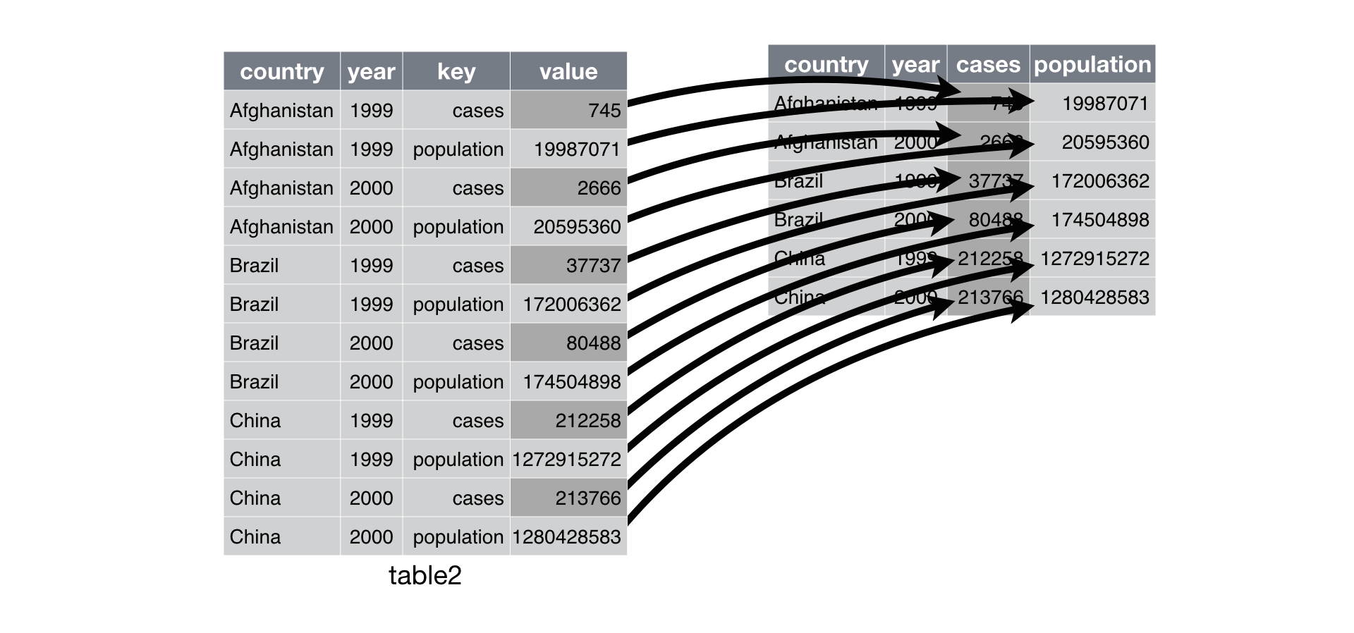
Pivot Longer

Source : R4DS - Tidy Data

Pivot Longer

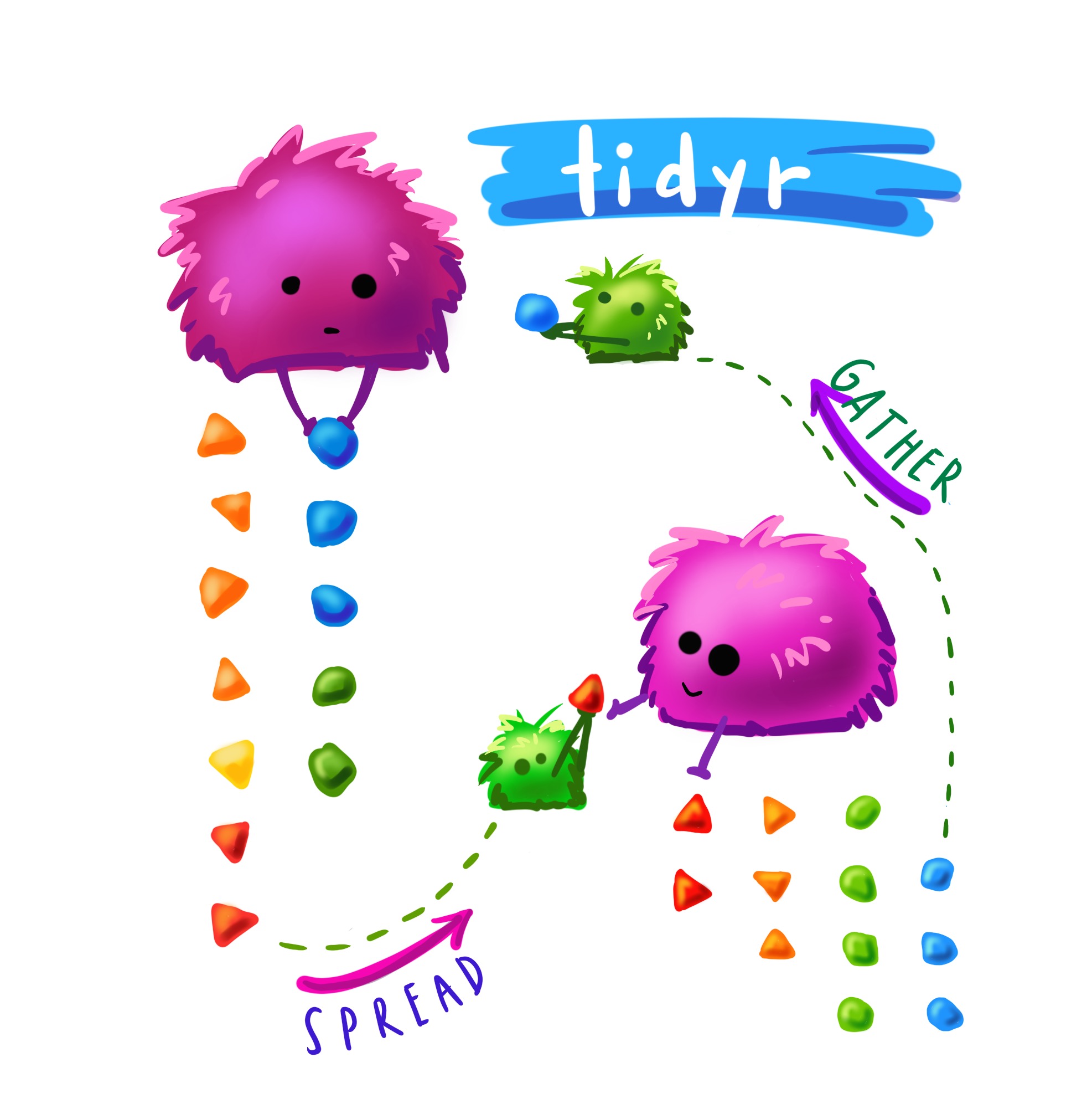
(Image from Alisson Horst, check her other stats illustrations here)

One cell contains multiple values

Now it’s clear that element contains more than one value.

For example: ba_mg_g_leachate is not a single values and could be split into:

element: ba.
unit: mg_g.
fraction: leachate.

Let’s split this column at the _ and reconstitute it in a tidy way

pangaea_tidy <- 
  pangaea_long %>% 
  separate(element, into = c('element', 'unit_num', 'unit_dem', 'fraction'), sep = '_') %>% 
  unite(col = 'unit', unit_num:unit_dem, sep = '/')

pangaea_tidy

# A tibble: 1,280 × 13
   event latit…¹ longi…² eleva…³ sampl…⁴ samp_…⁵ depth_m age_k…⁶ ca_co…⁷ element
   <chr>   <dbl>   <dbl>   <dbl> <chr>   <chr>     <dbl>   <dbl>   <dbl> <chr>  
 1 SL73…    39.7    24.5    -339 SL73-1  non-S1   0.0045    1.66    61.5 ba     
 2 SL73…    39.7    24.5    -339 SL73-1  non-S1   0.0045    1.66    61.5 sr     
 3 SL73…    39.7    24.5    -339 SL73-1  non-S1   0.0045    1.66    61.5 ca     
 4 SL73…    39.7    24.5    -339 SL73-1  non-S1   0.0045    1.66    61.5 al     
 5 SL73…    39.7    24.5    -339 SL73-1  non-S1   0.0045    1.66    61.5 fe     
 6 SL73…    39.7    24.5    -339 SL73-1  non-S1   0.0045    1.66    61.5 ba     
 7 SL73…    39.7    24.5    -339 SL73-1  non-S1   0.0045    1.66    61.5 sr     
 8 SL73…    39.7    24.5    -339 SL73-1  non-S1   0.0045    1.66    61.5 ca     
 9 SL73…    39.7    24.5    -339 SL73-1  non-S1   0.0045    1.66    61.5 al     
10 SL73…    39.7    24.5    -339 SL73-1  non-S1   0.0045    1.66    61.5 fe     
# … with 1,270 more rows, 3 more variables: unit <chr>, fraction <chr>,
#   concentration <dbl>, and abbreviated variable names ¹latitude, ²longitude,
#   ³elevation_m, ⁴sample_label_barite_sr, ⁵samp_type, ⁶age_ka_bp,
#   ⁷ca_co3_percent
# ℹ Use `print(n = ...)` to see more rows, and `colnames()` to see all variable names

pangaea_tidy %>% glimpse()

Rows: 1,280
Columns: 13
$ event                  <chr> "SL73BC", "SL73BC", "SL73BC", "SL73BC", "SL73BC…
$ latitude               <dbl> 39.6617, 39.6617, 39.6617, 39.6617, 39.6617, 39…
$ longitude              <dbl> 24.5117, 24.5117, 24.5117, 24.5117, 24.5117, 24…
$ elevation_m            <dbl> -339, -339, -339, -339, -339, -339, -339, -339,…
$ sample_label_barite_sr <chr> "SL73-1", "SL73-1", "SL73-1", "SL73-1", "SL73-1…
$ samp_type              <chr> "non-S1", "non-S1", "non-S1", "non-S1", "non-S1…
$ depth_m                <dbl> 0.0045, 0.0045, 0.0045, 0.0045, 0.0045, 0.0045,…
$ age_ka_bp              <dbl> 1.66, 1.66, 1.66, 1.66, 1.66, 1.66, 1.66, 1.66,…
$ ca_co3_percent         <dbl> 61.5, 61.5, 61.5, 61.5, 61.5, 61.5, 61.5, 61.5,…
$ element                <chr> "ba", "sr", "ca", "al", "fe", "ba", "sr", "ca",…
$ unit                   <chr> "mg/g", "mg/g", "mg/g", "mg/g", "mg/g", "mg/g",…
$ fraction               <chr> "leachate", "leachate", "leachate", "leachate",…
$ concentration          <dbl> 72.6, 767.0, 188951.9, 10612.7, 5935.0, 171.0, …

And let’s fix the measurement unit

Remember that janitor transformed µ into m?

pangea_tidy <- 
  pangaea_tidy %>% 
  mutate(unit = unit %>% str_replace('m', 'µ'))

pangaea_tidy

# A tibble: 1,280 × 13
   event latit…¹ longi…² eleva…³ sampl…⁴ samp_…⁵ depth_m age_k…⁶ ca_co…⁷ element
   <chr>   <dbl>   <dbl>   <dbl> <chr>   <chr>     <dbl>   <dbl>   <dbl> <chr>  
 1 SL73…    39.7    24.5    -339 SL73-1  non-S1   0.0045    1.66    61.5 ba     
 2 SL73…    39.7    24.5    -339 SL73-1  non-S1   0.0045    1.66    61.5 sr     
 3 SL73…    39.7    24.5    -339 SL73-1  non-S1   0.0045    1.66    61.5 ca     
 4 SL73…    39.7    24.5    -339 SL73-1  non-S1   0.0045    1.66    61.5 al     
 5 SL73…    39.7    24.5    -339 SL73-1  non-S1   0.0045    1.66    61.5 fe     
 6 SL73…    39.7    24.5    -339 SL73-1  non-S1   0.0045    1.66    61.5 ba     
 7 SL73…    39.7    24.5    -339 SL73-1  non-S1   0.0045    1.66    61.5 sr     
 8 SL73…    39.7    24.5    -339 SL73-1  non-S1   0.0045    1.66    61.5 ca     
 9 SL73…    39.7    24.5    -339 SL73-1  non-S1   0.0045    1.66    61.5 al     
10 SL73…    39.7    24.5    -339 SL73-1  non-S1   0.0045    1.66    61.5 fe     
# … with 1,270 more rows, 3 more variables: unit <chr>, fraction <chr>,
#   concentration <dbl>, and abbreviated variable names ¹latitude, ²longitude,
#   ³elevation_m, ⁴sample_label_barite_sr, ⁵samp_type, ⁶age_ka_bp,
#   ⁷ca_co3_percent
# ℹ Use `print(n = ...)` to see more rows, and `colnames()` to see all variable names

Data can take many shapes

pangaea_also_tidy <- 
  pangaea_tidy %>% 
  pivot_wider(names_from = 'element', values_from = 'fraction') 
  
pangaea_also_tidy

# A tibble: 1,280 × 16
   event  latitude longi…¹ eleva…² sampl…³ samp_…⁴ depth_m age_k…⁵ ca_co…⁶ unit 
   <chr>     <dbl>   <dbl>   <dbl> <chr>   <chr>     <dbl>   <dbl>   <dbl> <chr>
 1 SL73BC     39.7    24.5    -339 SL73-1  non-S1   0.0045    1.66    61.5 mg/g 
 2 SL73BC     39.7    24.5    -339 SL73-1  non-S1   0.0045    1.66    61.5 mg/g 
 3 SL73BC     39.7    24.5    -339 SL73-1  non-S1   0.0045    1.66    61.5 mg/g 
 4 SL73BC     39.7    24.5    -339 SL73-1  non-S1   0.0045    1.66    61.5 mg/g 
 5 SL73BC     39.7    24.5    -339 SL73-1  non-S1   0.0045    1.66    61.5 mg/g 
 6 SL73BC     39.7    24.5    -339 SL73-1  non-S1   0.0045    1.66    61.5 mg/g 
 7 SL73BC     39.7    24.5    -339 SL73-1  non-S1   0.0045    1.66    61.5 mg/g 
 8 SL73BC     39.7    24.5    -339 SL73-1  non-S1   0.0045    1.66    61.5 mg/g 
 9 SL73BC     39.7    24.5    -339 SL73-1  non-S1   0.0045    1.66    61.5 mg/g 
10 SL73BC     39.7    24.5    -339 SL73-1  non-S1   0.0045    1.66    61.5 mg/g 
# … with 1,270 more rows, 6 more variables: concentration <dbl>, ba <chr>,
#   sr <chr>, ca <chr>, al <chr>, fe <chr>, and abbreviated variable names
#   ¹longitude, ²elevation_m, ³sample_label_barite_sr, ⁴samp_type, ⁵age_ka_bp,
#   ⁶ca_co3_percent
# ℹ Use `print(n = ...)` to see more rows, and `colnames()` to see all variable names

pangaea_also_tidy %>% glimpse()

Rows: 1,280
Columns: 16
$ event                  <chr> "SL73BC", "SL73BC", "SL73BC", "SL73BC", "SL73BC…
$ latitude               <dbl> 39.6617, 39.6617, 39.6617, 39.6617, 39.6617, 39…
$ longitude              <dbl> 24.5117, 24.5117, 24.5117, 24.5117, 24.5117, 24…
$ elevation_m            <dbl> -339, -339, -339, -339, -339, -339, -339, -339,…
$ sample_label_barite_sr <chr> "SL73-1", "SL73-1", "SL73-1", "SL73-1", "SL73-1…
$ samp_type              <chr> "non-S1", "non-S1", "non-S1", "non-S1", "non-S1…
$ depth_m                <dbl> 0.0045, 0.0045, 0.0045, 0.0045, 0.0045, 0.0045,…
$ age_ka_bp              <dbl> 1.66, 1.66, 1.66, 1.66, 1.66, 1.66, 1.66, 1.66,…
$ ca_co3_percent         <dbl> 61.5, 61.5, 61.5, 61.5, 61.5, 61.5, 61.5, 61.5,…
$ unit                   <chr> "mg/g", "mg/g", "mg/g", "mg/g", "mg/g", "mg/g",…
$ concentration          <dbl> 72.6, 767.0, 188951.9, 10612.7, 5935.0, 171.0, …
$ ba                     <chr> "leachate", NA, NA, NA, NA, "residue", NA, NA, …
$ sr                     <chr> NA, "leachate", NA, NA, NA, NA, "residue", NA, …
$ ca                     <chr> NA, NA, "leachate", NA, NA, NA, NA, "residue", …
$ al                     <chr> NA, NA, NA, "leachate", NA, NA, NA, NA, "residu…
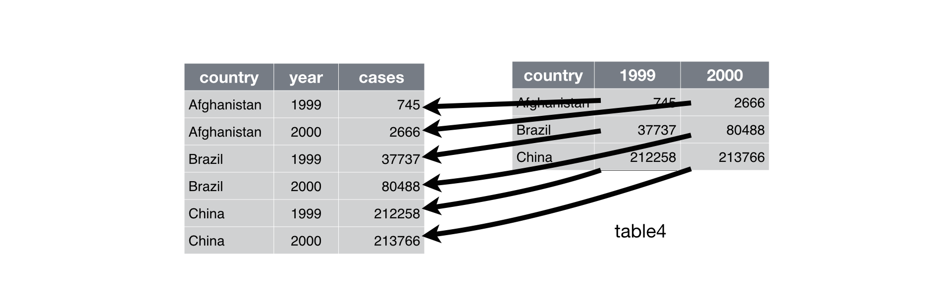
$ fe                     <chr> NA, NA, NA, NA, "leachate", NA, NA, NA, NA, "re…

Pivot Wider

Source : R4DS - Tidy Data

Exercise

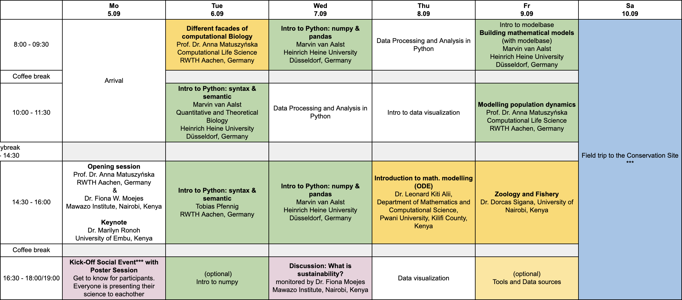
Tidy last week’s schedule.

Clean and Tidy Data

Tidy Data

Which Dataset is Tidy?

Which Dataset is Tidy?

Semantics of (tidy) Data

Tools: Tidy data with Tidyr

Let’s tidy the data from Pangaea

Pangea Data

Clean the column names with Janitor

Place fixed variables in the first columns

There are values stored in the column names

Pivot Longer

Pivot Longer

One cell contains multiple values

And let’s fix the measurement unit

Data can take many shapes

Pivot Wider

Exercise

Clean the column names with `Janitor`