Robust Summary Statistics

Otho Mantegazza

Summary Statistics

Concise summaries

When we mentioned the boxplot, we talked about robust summary statistics. First of all, what is a summary statistic?

A Summary statistic describes a property of a distribution in one single number.

For example:

• The mean represents the central tendency of a distribution.
• The standard deviation represents its dispersion.

None of these statistics is robust toward outliers.

Mean and Standard Deviation

- Mean

\(mean(x) = \frac{1}{n} \sum_{i=i}^{n} x_{i}\)

- Standatrd Deviation

\(SD = \sqrt{\frac{1}{N-1} \sum_{i=1}^N \left(x_i - \bar{x}\right)^2}\)

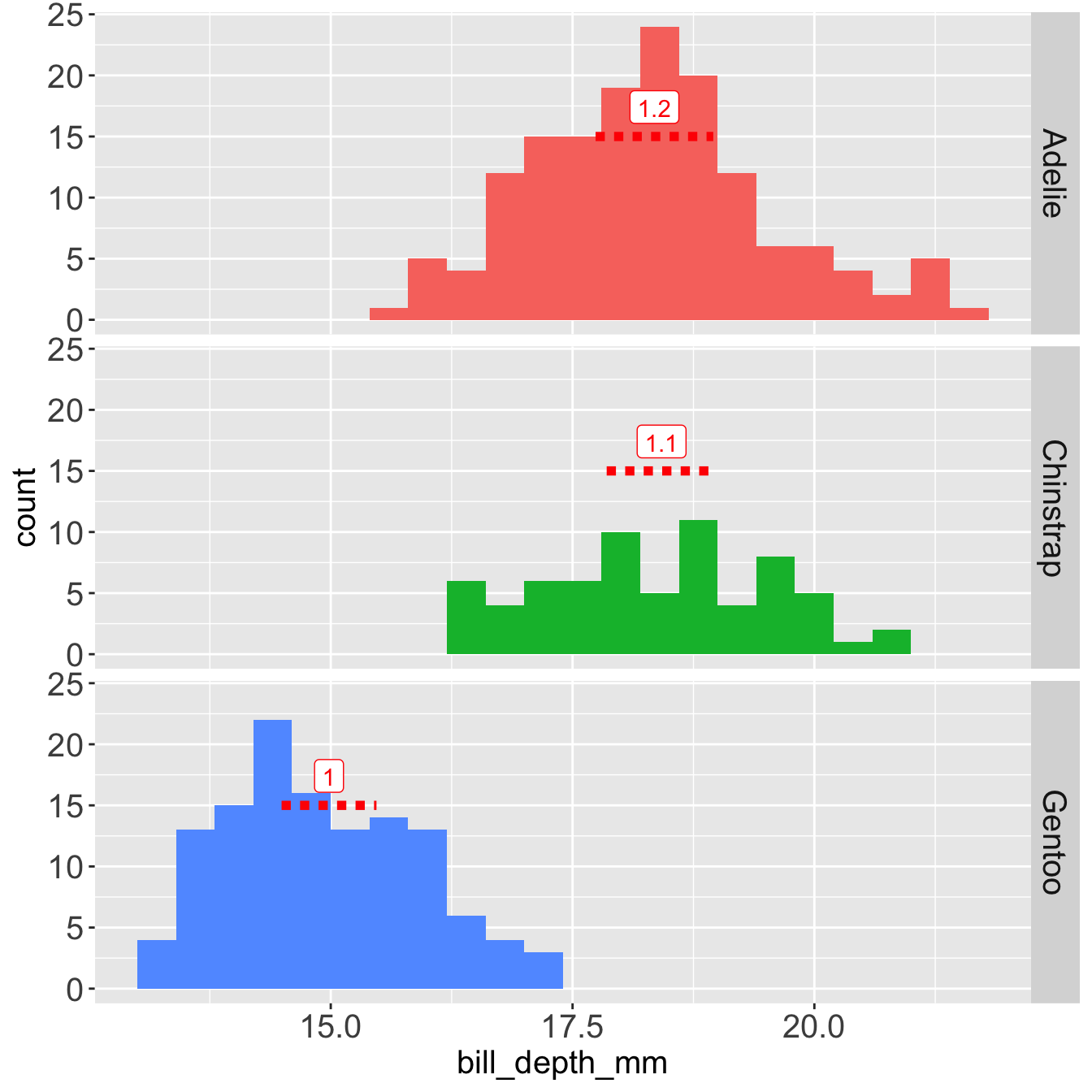
Mean and SD are not robust to outlier

What if I’m distracted and forget to write a comma when I collect the data.

penguins$bill_depth_mm %>% range(na.rm = T)

[1] 13.1 21.5

With this snipped we multiply the max value of bill_depth_mm by 10.

penguins_bad <- 
  penguins %>% 
    mutate(
      bill_depth_mm = bill_depth_mm %>% 
        {
          if_else(. == max(., na.rm = T),
                    true = .*10,
                    false = .)
        }
    )

With this chunk of code I’ve added an outlier at in the variable bill_depth_mm at 215 mm. Let’s see what happens.

Mean and SD with an outlier at 215 mm

I’ve added an outlier to the Adelie species, let’s see what happens graphically

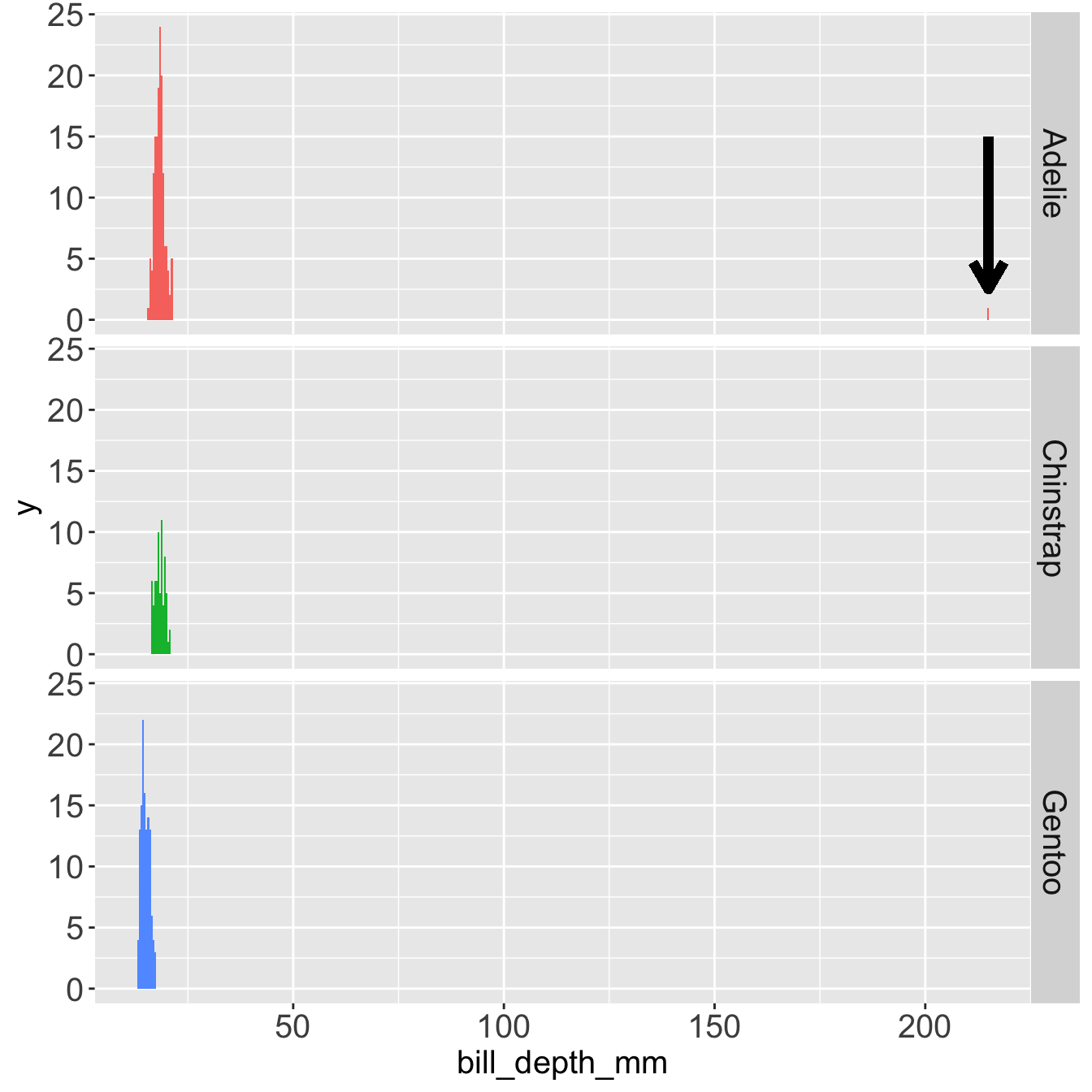
In the next plots I will not represent the outlier graphically because it stretches the x axis too much.

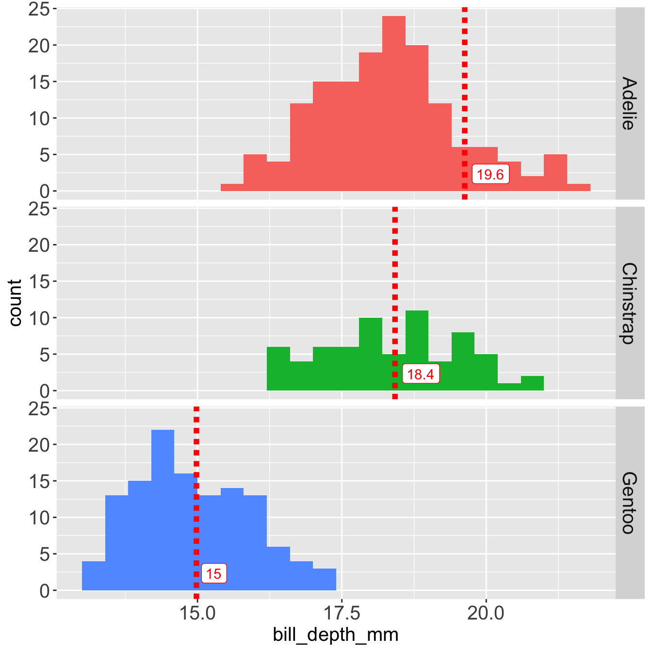
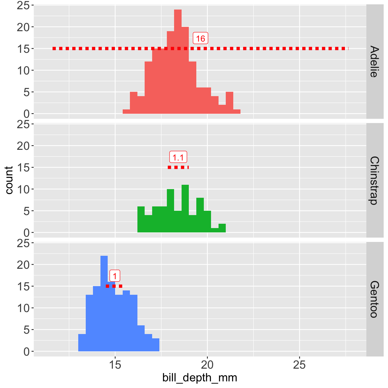
Mean and SD are heavily influenced by the outlier.

The mean of Adelie is influenced by the outlier at 215 mm

The SD of Adelie is influenced by the outlier 215 mm

Robust Summary Statistics

Median and Interquartile Range (IQR)

Median

The median represents a the central tendency of a distribution, it is the value that splits the bigger 50% (half) of the data from the smaller half.

Interquartile Range (IQR)

The IQR range represents how a distribution is dispersed, it is the range between the 1st and the 3rd quartile.

• The 1st quartile splits the smaller 25% of a distribution from the rest.
• The 3rd quartile splits the bigger 75% of a distribution from the rest.

Median and IQR without outlier

- Median

- IQR

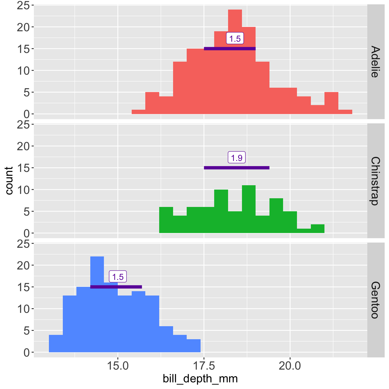
Median and IQR with an outlier at 215 mm

The median is not influenced by the outlier at 215 mm

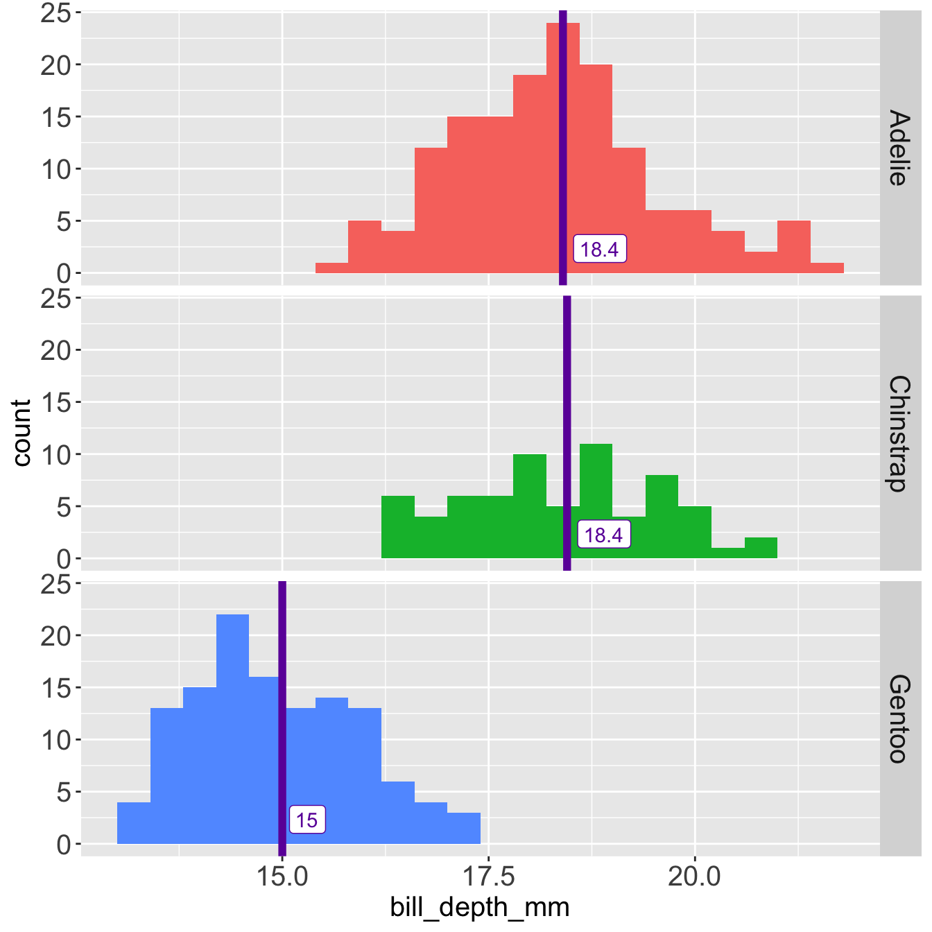
The median is not influenced by the outlier at 215 mm

References

Referece - Summaries

Summary statistic without outlier.

penguins_summarized

# A tibble: 3 × 8
  species       m    sd   med    q1    q3   iqr   mad
  <fct>     <dbl> <dbl> <dbl> <dbl> <dbl> <dbl> <dbl>
1 Adelie     18.3 1.22   18.4  17.5  19    1.5   1.19
2 Chinstrap  18.4 1.14   18.4  17.5  19.4  1.90  1.41
3 Gentoo     15.0 0.981  15    14.2  15.7  1.5   1.19

Summary statistic with an outlier at 215 mm.

penguins_bad_summarized

# A tibble: 3 × 8
  species       m     sd   med    q1    q3   iqr   mad
  <fct>     <dbl>  <dbl> <dbl> <dbl> <dbl> <dbl> <dbl>
1 Adelie     19.6 16.0    18.4  17.5  19    1.5   1.19
2 Chinstrap  18.4  1.14   18.4  17.5  19.4  1.90  1.41
3 Gentoo     15.0  0.981  15    14.2  15.7  1.5   1.19

Reference - Functions

• Mean: mean()
• Standard Deviation: sd()
• Median: median() or quantile()['50%']
• 1st quartile: quantile()['25%']
• 3rd quartile: quantile()['75%']
• IQR: iqr()

Use na.rm = TRUE with all those function to ignore missing values.

Take home

• When we have many data, we often have to reduce them to simple indicators with summary statistics.

• No statisitic is perfect, some, such as mean and standard deviation are more precise, but they “break” easilt if the data with “non-ideal” data.

• Others are such as median and IQR are simpler and less sophisticated, but are better at capturing the essence of the data in “non-ideal” situation, i.e. robust.

• The word robust is often use to describe statistical methods. It means that the method is unlikely to break when the data are not perfect and the condition are worse than ideal.

Read: Introduction to data science | Chapter 12 - Robust Summaries

Exercise

The storm dataset is loaded in R with the tidyverse. It stores attributes from hurricanes in the US over the years 1975-2020.

• What are the mean and the median wind speed?
• What are the mean and the median air pressure in the storm center?

Investigate the wind and pressure variables with histograms and boxplots, how are the data distributed? are there any outlier?

What if you stratify those two variables by status, do you see some interesting pattern?

Stratify the data by name, extract the 5 hurricanes with the highest mean wind speed the 5 hurricanes with highest median wind speed. Are they the same?